Flatland
Accelerate the learning – increase agents behavior at higher speed!
New changes related to flatland
TL:DR:
- I improved the performance of the Flatland environment by optimizing critical code paths using a profiler. These changes have been included in the latest Flatland release.
- I introduce a new observation builder,
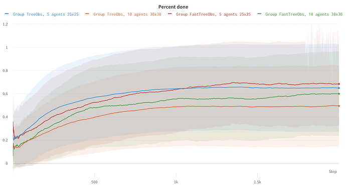
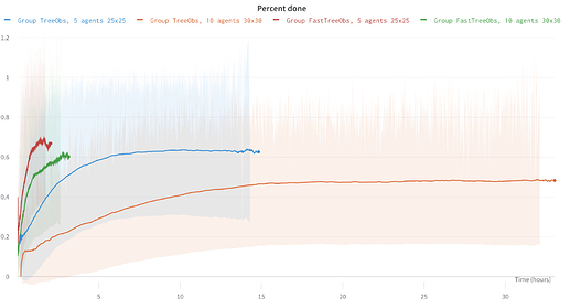
FastTreeObs, which performs many time faster than the default TreeObs and reaches better performance for RL-based agents. See the comparison below:FastTreeObsin red and green vs defaultTreeObsin blue and orange.- This new observation builder has already been added in the Starter kit in the
fast-tree-obsbranch! 5 use--use_extra_observation
I would like to share some of the things I’ve learnt while working with FLATland. I would also like to share some working experience in the field of mathematical optimization where I have been developing solutions for more than a decade, in the hope that these experiences might help to solve similarly complex problems.
One key issue with reinforcement learning is that to train agents we have to show hundreds of thousands of different variants. To do this in a reasonable amount of time we must have a fast environment. So to shorten the training time we can accelerate the FLATland environment by using faster computers or we can change the optimization model or the implementation of FLATland. Based on my experience you should not invest too much time accelerating code such as the FLATland core when working with early, naive optimisation models, such as RL agents and their observations. Doing core optimisations in general increases code complexity and it doesn’t make a big difference towards optimisation quality. Of course core optimisations allow you to train more episodes in fixed time. But I think this will not make a major difference to agents’ behavior or optimisation quality.
Nevertheless, I decided as a first step using a profiler to get a first insight into whether there are some low-hanging-fruits to optimize. This is cheap in doing and could make a first improvement. But I was aware that this can not make a big improvement in agents behavior after training. What I did was simply to run FLATland with a profiler. I profiled FLATland with yappi and analyzed the call graph. Within a very short time I found some expensive function calls in the core and as well in the build-in tree observation. I just focused on the most expensive ones. Then I found a better implementation and so I replaced just five numpy function calls. I used only pure python methods and I got the FLATland core accelerated by factors 3-4.
Which numpy functions are extremely expensive and should not be used in FLATland? The most expensive one is np.isclose. Thus I suggested replacing np.isclose with fast_isclose which is my pure python replacement. Next you take by using np.clip or np.argmax. Beside those three methods I worked out that two other methods have a major impact on the overall performance, thus I suggested also to replace equal for position comparison and count_nonzero for counting the number of possible transitions.
def fast_isclose(a, b, rtol):
    return (a < (b + rtol)) or (a < (b - rtol))


def fast_clip(position: (int, int), min_value: (int, int), max_value: (int, int)) -> bool:
    return (
        max(min_value[0], min(position[0], max_value[0])),
        max(min_value[1], min(position[1], max_value[1]))
    )


def fast_argmax(possible_transitions: (int, int, int, int)) -> bool:
    if possible_transitions[0] == 1:
        return 0
    if possible_transitions[1] == 1:
        return 1
    if possible_transitions[2] == 1:
        return 2
    return 3


def fast_position_equal(pos_1: (int, int), pos_2: (int, int)) -> bool:
    return pos_1[0] == pos_2[0] and pos_1[1] == pos_2[1]


def fast_count_nonzero(possible_transitions: (int, int, int, int)):
    return possible_transitions[0] + possible_transitions[1] + possible_transitions[2] + possible_transitions[3]
Those methods are now part of the latest FLATland release. Many thanks to the community to integrate them into FLATland core.
from time import time

import numpy as np
from flatland.envs.rail_env import fast_isclose


def print_timing(label, start_time, end_time):
    print("{:>10.4f}ms".format(1000 * (end_time - start_time)) + "\t" + label)


def check_isclose(nbr=100000):
    s = time()
    for x in range(nbr):
        fast_isclose(x, 0.0, rtol=1e-03)
    e = time()
    print_timing("fast_isclose", start_time=s, end_time=e)

    s = time()
    for x in range(nbr):
        np.isclose(x, 0.0, rtol=1e-03)
    e = time()
    print_timing("np.isclose", start_time=s, end_time=e)


if __name__ == "__main__":
    check_isclose()

#21.9455ms	fast_isclose
#2421.8295ms	np.isclose
This optimization makes it possible to train a reinforcement learning agent on FLATland much faster. But it made no difference in agents’ behavior! I think the whole community can now benefit from these code accelerations. That’s great. So the wave evaluation strategy with these optimizations enables to execute more scenarios in the limited time and so you all get higher reward.
But then I switch to the more interesting work – I like to understand what the agents can do and I like to understand how I can use these problem understanding to rewrite the observation model. So I focus most time on the model and the question of how we can reformulate the tree observation to improve agents behavior at higher calculation speed. This work is fun!
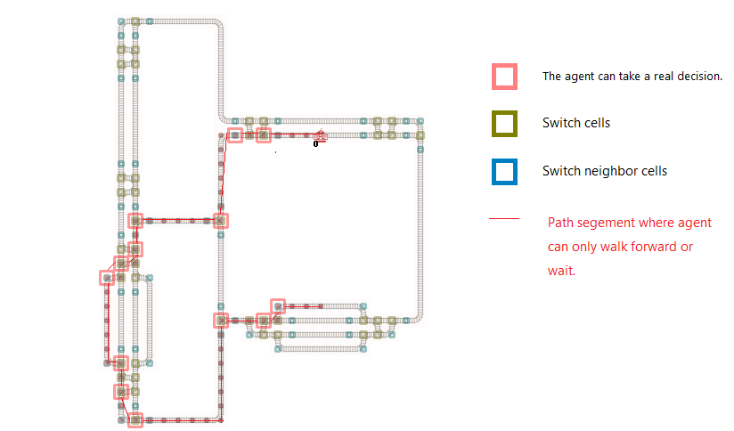
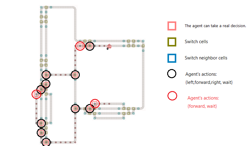
What observation I made while analyzing FLATland? I got that the agent’s action space is not at each cell the same. Thus the action space is locally different and might be used to better formulate the observation. The key question was to understand where an agent can freely choose the full action space and where an agent can only walk forward to optimize the reward.
Where agents can choose an action from full action space is where they can make a real decision. This is in general on a cell before a switch and on a cell which is a switch.
One cell before a switch (agent is looking toward the switch which is joining two tracks) the agent can only choose to wait or walk forward. All other actions don’t optimize the reward function. What is going on there? Two trains can change their ordering, A before B or B before A. For all other switches the agent has to walk at least one step and has to decide on the switch which track the train has to take. Thus on a switch the agent can only make a routing decision. In most cases the agent has to choose to continue walking on the shortest path to optimize the reward function. But he has to ensure that the chosen path will end at the target and has to avoid deadlocks.
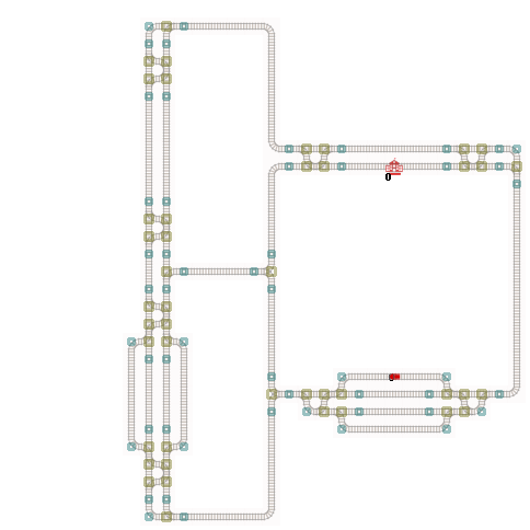
What conceptual issue I believe is in the current observation:
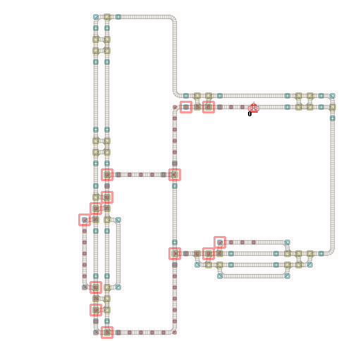
At the red box the agent can choose an action. The number of cells where agents can make real decisions is severely limited.
These findings where used to build a new observation builder. From experiments it shows that agent's behavior will not be worse than the Flatland-built-in tree observation.
My observation contains only 26 values:
# all values are [0,1]
# observation[0]  : 1 path towards target (direction 0) / otherwise 0 -> path is longer or there is no path
# observation[1]  : 1 path towards target (direction 1) / otherwise 0 -> path is longer or there is no path
# observation[2]  : 1 path towards target (direction 2) / otherwise 0 -> path is longer or there is no path
# observation[3]  : 1 path towards target (direction 3) / otherwise 0 -> path is longer or there is no path
# observation[4]  : int(agent.status == RailAgentStatus.READY_TO_DEPART)
# observation[5]  : int(agent.status == RailAgentStatus.ACTIVE)
# observation[6]  : int(agent.status == RailAgentStatus.DONE or agent.status == RailAgentStatus.DONE_REMOVED)
# observation[7]  : current agent is located at a switch, where it can take a routing decision
# observation[8]  : current agent is located at a cell, where it has to take a stop-or-go decision
# observation[9]  : current agent is located one step before/after a switch
# observation[10] : 1 if there is a path (track/branch) otherwise 0 (direction 0)
# observation[11] : 1 if there is a path (track/branch) otherwise 0 (direction 1)
# observation[12] : 1 if there is a path (track/branch) otherwise 0 (direction 2)
# observation[13] : 1 if there is a path (track/branch) otherwise 0 (direction 3)
# observation[14] : If there is a path with step (direction 0) and there is a agent with opposite direction -> 1
# observation[15] : If there is a path with step (direction 1) and there is a agent with opposite direction -> 1
# observation[16] : If there is a path with step (direction 2) and there is a agent with opposite direction -> 1
# observation[17] : If there is a path with step (direction 3) and there is a agent with opposite direction -> 1
# observation[18] : If there is a path with step (direction 0) and there is a agent with same direction -> 1
# observation[19] : If there is a path with step (direction 1) and there is a agent with same direction -> 1
# observation[20] : If there is a path with step (direction 2) and there is a agent with same direction -> 1
# observation[21] : If there is a path with step (direction 3) and there is a agent with same direction -> 1
# observation[22] : If there is a switch on the path which agent can not use -> 1
# observation[23] : If there is a switch on the path which agent can not use -> 1
# observation[24] : If there is a switch on the path which agent can not use -> 1
# observation[25] : If there is a switch on the path which agent can not use -> 1
At a switch the new observation explores similar to the tree observation. But it don’t branch at all switch the exploration. It only branchs at real decision points. The exploration stops when an other agent is encountered or breaks when it reaches the max allowed exploration depth. And of course it stops the exploration when the maximal branch depth is reached. Then it just aggregates the observations made during the exploration.
Here are some experimental results with FastTreeObs: using the starter kit DDDQN implementation. The new observation gets better results when looking at sample efficiency
Screenshot 2020-10-22 at 12.27.371868×1014 112 KB
However it’s when you look at the time efficiency that you see it’s true potential 

Content
Comments
You must login before you can post a comment.


